The Ultimate Guide To Implied Volatility

by Gavin in Blog, implied volatility

April 30, 2020 • 7 comments

Contents

• Introduction
• Option Volatility Explained
• Why Should You Care?
• Implied Volatility And Historical Volatility
• Implied Volatility And The Black Scholes Formula
• Implied Volatility Calculation
• Standard Deviation And Implied Volatility
• Standard Deviation For Shorter Time Periods
• Using Implied Volatility To Gain An Edge
• Volatility Analysis For A Portfolio Of Options
• Implied Volatility And Option Strategies
• FAQ
• Conclusion

Introduction

When first starting out, many beginner option traders are somewhat bamboozled by the concept of option implied volatility.

If you find yourself in this position, then don’t worry, you’re certainly not alone – and this article is here to help rectify the situation.

One thing you absolutely cannot do is ignore volatility and put it in the “too hard” basket.

Of all the different aspects of trading options that you need to grasp, this one is the most crucial.

Understanding volatility is not only crucial, but also a fascinating part of trading.

With stocks, you can make money if the stock moves up or down; but options provide such amazing flexibility, you can profit in a multitude of different environments.

Of course, with that flexibility comes more risk.

Take for example, the trader who buys a call option thinking the stock is going to rise.

The next day his stock rises, but his call option falls in price.

I’ve coached hundreds of options traders, and almost all beginners struggle to understand how this can happen.

The answer is: that the volatility of that option has dropped, resulting in a drop in price of the option.

This is just one example of how volatility can negatively impact the unwary trader.

Today, I’ll take a look at some of the important concepts surrounding option volatility and how you can use them to create profitable trades.

Option Volatility Explained

Option volatility is a key concept for option traders and even if you are a beginner, you should try to have at least a basic understanding.

Option volatility is reflected by the Greek symbol Vega, which is defined as the amount that the price of an option changes compared to a 1% change in volatility.

In other words, an options Vega is a measure of the impact of changes in the underlying volatility on the option price.

All else being equal (no movement in share price or interest rates, and no passage of time), option prices will increase if there is an increase in volatility, and decrease if there is a decrease in volatility.

Therefore, it stands to reason that buyers of options (those that are long either calls or puts), will benefit from increased volatility, and sellers will benefit from decreased volatility.

The same can be said for spreads – debit spreads (trades where you pay to place the trade) will benefit from increased volatility, while credit spreads (where you receive money after placing the trade) will benefit from decreased volatility.

Here is a theoretical example to demonstrate the idea. Let’s look at a stock priced at 50. Consider a 6-month call option with a strike price of 50:

If the implied volatility is 90, the option price is $12.50

If the implied volatility is 50, the option price is $7.25

If the implied volatility is 30, the option price is $4.50

This shows you that, the higher the implied volatility, the higher the option price.

Why Should You Care?

One of the main reasons for needing to understand option volatility is that it will allow you to evaluate whether options are cheap or expensive, by comparing Implied Volatility (IV) with Historical Volatility (HV).

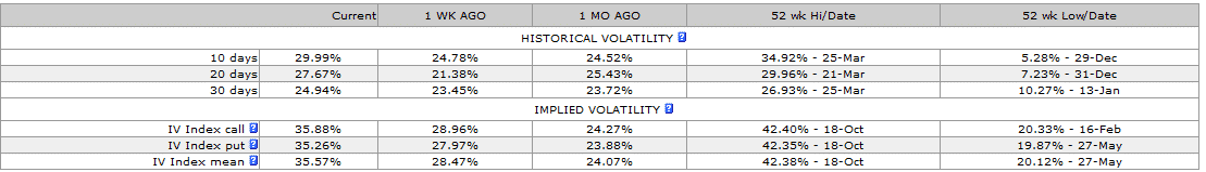
Below is an example of the Historical Volatility and Implied Volatility for AAPL.

You can get this data easily, and for free, from www.ivolatility.com.

You can see that at the time, AAPL’s Historical Volatility was 25-30% for the last 10-30 days, and that the current level of Implied Volatility is around 35%.

This shows you that traders were expecting big moves in AAPL going forward.

You can also see that the current levels of IV are much closer to the 52-week high than the 52-week low.

This indicates that this was potentially a good time to look at strategies that benefit from a fall in implied volatility.

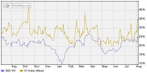
Here we are looking at this same information shown graphically. You can see there was a huge spike in mid-October. This coincided with a 6% drop in AAPL stock price.

Drops like this cause investors to become fearful, and this heightened level of fear is a great chance for options traders to pick up extra premium via net selling strategies such as credit spreads.

Or, if you were a holder of AAPL stock, you could use the volatility spike as a good time to sell some covered calls and pick up more income than you usually would for this strategy.

Generally, when you see IV spikes like this, they are short-lived, but be aware that things can and do get worse, such as in 2008.

Don’t just assume that volatility will return to normal levels within a few days or weeks.

Implied Volatility And Historical Volatility

Historical Volatility is calculated by measuring the past price movement of a stock.

It is a known figure as it is based on past data.

I won’t go into the details of how to calculate Historical Volatility, as it is very easy to do in Excel.

The data is readily available for you, so you generally will not need to calculate it yourself.

The main point is that in general, stocks that have had large price swings in the past will have high levels of Historical Volatility.

As options traders, we are more interested in how volatile a stock is likely to be during the duration of our trade.

Historical Volatility will give some guide to how volatile a stock is, but that is no way to predict future volatility.

The best we can do is estimate it – and this is where Implied Volatility comes in.

Implied Volatility is an estimate, made by professional traders and market makers, of the future volatility of a stock.

Access 9 Free Option Books

It is a key input in options pricing models.

The Black Scholes model is the most popular pricing model based on certain inputs, of which volatility is the most subjective (as future volatility cannot be known).

It therefore gives us the greatest chance to exploit our view of volatility compared to other traders.

Implied Volatility takes into account any events that are known to be occurring during the lifetime of the option that may have a significant impact on the price of the underlying stock.

This could include an earnings announcement, or the release of drug trial results for a pharmaceutical company, for example.

The current state of the general market is also incorporated in Implied Volatility.

If markets are calm, volatility estimates are low, but during times of market stress, volatility estimates will be raised.

One very simple way to keep an eye on the general market levels of volatility is to monitor the VIX Index, which I will discuss in detail shortly.

Implied Volatility Calculation And The Black Scholes Formula

In 1973, Fischer Black and Myron Scholes composed a paper that gave their interpretation on how to price the premium of a stock option.

The original piece priced the premium of a European call or put ignoring dividends.

Black and Scholes were awarded the Nobel Prize for economics in 1997, along with Robert Merton, who made a number of additional contributions to options pricing.

The calculation is based on the idea that a call and a put determine the likelihood that the underlying stock will be “in the money” prior to the expiration date of the option.

The expiration date is the day the option no longer exists, and the right to purchase or sell the underlying security expires.

A European-style option is one that can only be exercised on the expiration date.

This means that a trader cannot exercise prior to expiration, but can still sell the option for a gain or loss before the expiration date.

To price an option, the Black Scholes model needs a number of inputs, which include:

-The current underlying price of the security

-The current prevailing short term interest rates

-The strike price of the options

-The time until expiration

-The Implied Volatility for the option.

The math behind the pricing model is relatively complicated, but today the model is freely available and using it does not require the trader understands the math.

The key input that traders need to focus on is the Implied Volatility.

All other inputs are known inputs. Implied Volatility is the market’s estimate of how far and fast the stock will move, and is completely subjective.

This is where traders have the opportunity to gain an edge.

If you think the market is underestimating volatility, you buy options.

If you think the market is overestimating volatility, you sell options.

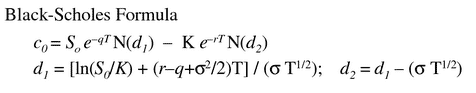
Below is the Black Scholes formula in case you are interested, but in all likelihood you will never need this.

Implied Volatility Calculation

These days you never have to calculate out the Black Scholes formula manually.

There are also some fantastic tools around that help you calculate and run various scenarios for Implied Volatility.

One of these was created by Samir at Investexcel.net.

I really love this tool, and you can download a copy here.

You know you’re a nerd when you get excited about an Excel file….!

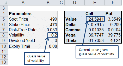
With the spreadsheet you can alter the volatility rate, and then calculate the new call and put values. As I said, very cool….

Note that the Excel file must be used as a 97-2003 workbook.

You can adjust any variable in the parameters section.

For example, your scenario might be that you expect volatility to rise from 0.20 to 0.23 over the next 5 days.

You would change the volatility value and also the expiry time to take into account the passage of 5 days, then, using the Goal Seek function in Excel, calculate the option values.

Note that this is designed for European options, not American options.

Here are the instructions for using the spreadsheet, as provided by Samir.

It might seem complicated at first glance, but really it is very simple; so even if you are not an Excel whiz, you should still be able to figure it out.

Step 1. In the spreadsheet, enter the Spot (stock) Price, Strike Price, Risk Free Rate and Expiry Time. Also, enter an initial guess value for the volatility (this will give you an initial call price, which is refined in the next step).

Step 2. Go to Data>What If Analysis>Goal Seek. Set the Call value to 30 (cell E5 in the spreadsheet) by changing the volatility (cell B8 in the spreadsheet).

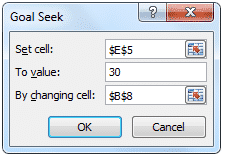
Step 3. Click OK.

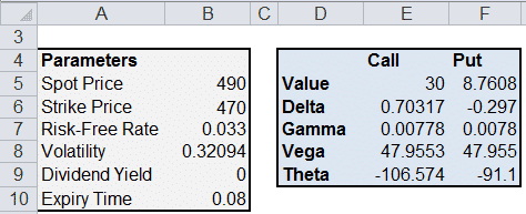
You should find that volatility has been updated to 0.32 to reflect the desired call price of 30.

The spreadsheet also gives you other, cool data such as the change in greeks for a given change in volatility, time to expiry, stock price, etc.

Simply awesome stuff. Tip of the cap to you, Samir!

Standard Deviation And Implied Volatility

In layman terms, Implied Volatility is the market opinion of the potential movement or range of a stock over the following 12-month period.

As you can probably deduce, a stock with a high Implied Volatility is expected to have large swings in price, while a stock with low volatility is expected to have small swings.

Implied Volatility is considered to be more important than Historical Volatility because it takes into account all factors, such as earnings, anticipated news and product releases.

Of course, there are always unanticipated events which come out of nowhere. These can never be priced in – but hey, trading would be boring otherwise, right?

To illustrate, let’s look at some examples.

The image below shows the Historical Volatility (blue line) and the Implied Volatility (gold line) of GOOG stock from February 2013 to February 2014.

There are a few things to note here.

Firstly, the red circles highlight times when Implied Volatility gradually rose up and then fell off a cliff.

This is a very common occurrence with stocks, and often occurs in the lead-up to earnings announcements.

Earnings are a great unknown for a stock, which can experience a huge move either way after the announcement, when the uncertainty surrounding the announcement is gone and Implied Volatility collapses.

Looking at the first red circle, you can see that Implied Volatility was around 27% leading into an earnings announcement, indicating that traders were expecting the stock to move within a 27% range over the following 12 months.

The second thing to note is the green circle.

On October 17th, GOOG announced blowout earnings and rose 14% the following day.

This is the reason for the huge spike in Historical Volatility, as the 14% move came into the calculation.

Thirty days later, when the 14% rise drops out of the calculation, the Historical Volatility comes back down to more normal levels.

You can see that around the same time, Implied Volatility drops from 27% down to 16% as the uncertainty around the earnings announcement is removed.

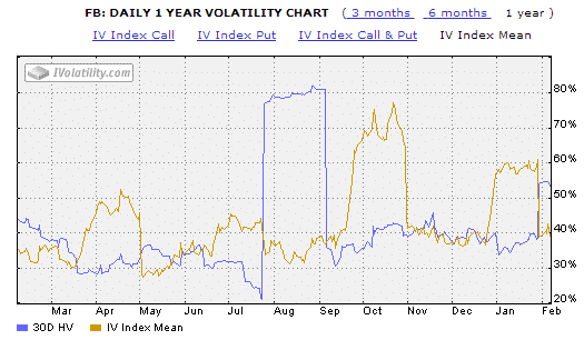
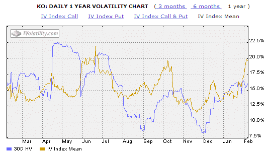
Now, let’s compare the Implied Volatility for FB and KO.

Get Your Free Put Selling Calculator

One is a high-flying tech stock and recent IPO, and the other is a stable, well established business in the consumer staples sector.

As you would expect, traders are expecting much bigger moves in FB, with Implied Volatility ranging from 29% to 78%.

Compare that with KO, which has an Implied Volatility range of 11-22%.

To understand how we can use standard deviation in our trading, we need to take a very brief trip back to our senior year math class and talk about normal distribution.

A normal distribution is sometimes called a “bell curve”, because of its shape; the underlying assumption is that prices have an equal chance of occurring above or below the center point (also known as the “average” or “mean”).

The Black Scholes model relies on a normal distribution, which is one of its limitations.

As we know, financial markets are anything but “normal” and have a propensity for what are known as “fat tails” (or “outliers” or “Black Swan events” if you prefer).

The other flaw with using a normal distribution assumption is the belief that prices have an equal chance of occurring above or below the mean.

A stock can only go to zero on the downside but can theoretically go to infinity on the upside.

Therefore, there are many more possible outcomes to the upside.

In any case, we will use the normal distribution for simplicity’s sake, but keep in mind these limitations.

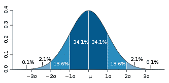
Taking a look at a standard bell curve, we can see that price will fall within a one standard deviation range 68% of the time; two standard deviation range 95% of the time; and a three standard deviation move 99.7% of the time.

Let’s take as an example a stock trading at $100 with Implied Volatility of 20%.

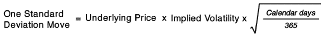
With this, we can calculate a one standard deviation move in the stock by taking the price multiplied by the Implied Volatility.

This tells us a one standard deviation move in this stock is $20, and that over the following 12 months, this stock has, roughly, a 68% chance of staying in that range.

Do you see where I’m going with this?

How could you apply this to a strategy like Iron Condors?

A one standard deviation move to the upside would put the stock at $120, and to the downside, at $80.

A two standard deviation move to the upside would put the stock at $140, and to the downside it would be at $60.

A three standard deviation move to the upside would put the stock at $160, and to the downside it would be at $40.

In other words, over the following 12 months, we can expect this stock to stay between $60 and $140 roughly 95% of the time.

However, as I mentioned earlier, the stock market has a propensity to experience fat tails, and trade outside of the 2 and 3 standard deviation moves more often than the normal distribution would suggest.

Think Lehman Brothers, Bear Sterns, etc.

Does this mean we should throw the idea of standard deviation out the window?

No, not necessarily.

Standard deviation gives us a very good estimate of where market participants think a stock will trade over the next 12 months based on their input for the level of Implied Volatility.

It’s your role to decide whether that assumption is too high or too low.

Increasing the Implied Volatility input into the pricing model will widen the standard deviations, while lowering your estimate of Implied Volatility will see the standard deviation ranges narrow.

Standard Deviation For Shorter Time Periods

It’s all well and good estimating a stock’s range over 12 months, but not many people trade 12-month options. Most people are interested in where a stock might trade over a one-week or one-month time frame.

Luckily, there is a very simply formula to convert the standard deviation calculation to factor in any time period.

I created a helpful spreadsheet that will do everything for you with only a couple of manual inputs; you can download it from here.

When you open the spreadsheet, simply update the formulas in the yellow cells – namely stock price, Implied Volatility and the expiry date.

It’s usually considered slightly more accurate to use the number of trading days in a year (252) rather than 365, which will yield slightly different results.

It’s up to you which you prefer to use.

Note that my spreadsheet uses 365.

If you need help changing it, just email me at [email protected].

It’s always easier to follow these things using an example, so let’s take our $100 stock with an Implied Volatility of 20% again, and look at how a one standard deviation move would look over a 30, 60 and 90 day time period.

30 Day, One Standard Deviation

The formula to calculate the one standard deviation move would be:

$100 x 0.20 x (SQRT (30/365)) = 5.73

Therefore, one standard deviation move for this stock over the course of 30 days would put it at $94.27 or $105.73. This is the range that we can expect the stock to stay within 68% of the time.

Out of interest, if we change calendar days to the number of trading days in a year, this is the result:

$100 x 0.20 x (SQRT (30/252)) = 6.90

The expected range is $93.10 to $106.90. You can see that using trading days is the more conservative assumption, so you may prefer to use this model.

60 Day, One Standard Deviation

The calculation for the 60 day, one standard deviation move using both models is shown below:

$100 x 0.20 x (SQRT (60/365)) = 8.11

$100 x 0.20 x (SQRT (60/252)) = 9.76

90 Day, One Standard Deviation

The calculation for the 90 day, one standard deviation move using both models is shown below:

$100 x 0.20 x (SQRT (90/365)) = 9.93

$100 x 0.20 x (SQRT (90/252)) = 11.95

If you have downloaded the standard deviation calculator spreadsheet, you will notice that there are two tabs: one for the 365-day calculation and another for the 252-day calculation.

If you have any issues, shoot me an email at [email protected]

You may have noticed that the further out in time you go, the larger the expected range. This makes sense, as the stock has a greater amount of time in which to make a move.

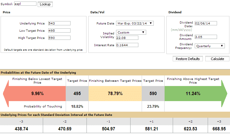
AAPL Example

Theoretical examples are fine, but let’s apply this to real world trading and see what information we can garner.

On February 13th, 2014, AAPL was trading at $543, with Implied Volatility at 22.08%.

The March 21st options were 36 days from expiry, so we will use them for this example.

The one standard deviation range for AAPL between February 13th and March 21st, is as follows:

$543 x 0.2208 x (SQRT (36/365)) = $37.65

Or

$543 x 0.2208 x (SQRT (36/252)) = $45.32

Taking the conservative estimate, let’s assume we want to trade an Iron Condor and place our short strikes slightly outside the one standard deviation range.

This gives us a choice of strikes around $495 and $590.

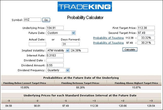
These days, a lot of brokers have probability calculators that do all the heavy lifting for you. Here are a couple of examples:

TRADE KING

OPTIONSHOUSE

Using Implied Volatility To Gain An Edge

Gaining an edge in the markets is harder than ever these days, with the advent of better technology, faster trading and easier access for the general public.

However, with your new-found knowledge of option volatility, you now have an advantage over 95% of the other participants in the market.

So how can you take advantage of that and create an edge?

The way I like to use Implied Volatility to gain an edge is to base some of my trade entry rules on certain levels of Implied Volatility.

The basic premise is that when volatility is high, you want to be leaning towards short volatility trades; and when volatility is low, you want to lean towards long volatility trades.

Pretty simple, right?

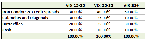
For example, in this low volatility environment of the last few years, you might set up a portfolio allocation similar to this:

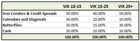
In this example, you can see that we’re allocating 50% to short Vega trades when the VIX is low; and 80% when the VIX is high.

We always like to keep some cash on hand in order to make adjustments.

Of course, you would need to adjust this for the market environment of the day.

This allocation probably wouldn’t have been appropriate back in the higher volatility days of 2008-2009. During those years, an allocation such as this would have made more sense:

Here you can see that the allocations are exactly the same, but the VIX levels, where the changes in allocation take place, are different. It is important to know whether you are in a low volatility environment, such as 2012-2013, or a high volatility environment like 2008-2009, and adjust your strategy allocation accordingly.

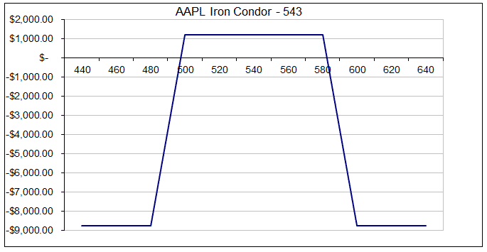
Let’s look at an example, Iron Condor trade, and see how it would perform assuming our opinion on where volatility was heading proved to be correct.

Date:   February 14th, 2014

Trade Details: AAPL Iron Condor

Current Price: $543

Buy 10 AAPL March 21st 485 puts @ 0.92

Sell 10 AAPL March 21st 495 puts @ 1.52

Sell 10 AAPL March 21st 590 calls @ 1.80

Buy 10 AAPL March 21st 600 calls @ 1.17

Premium: $1,230 Net Credit

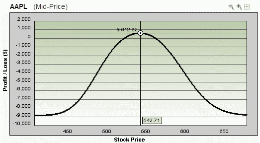
Here’s how the trade looks 10 days in, assuming a 10% relative drop in volatility.

You can see that it really pays to learn to understand volatility.

In this trade example, you’ve made half the potential profit in only 10 days, mostly thanks to the drop in volatility.

The other way to exploit an edge using volatility is by structuring your portfolio so that it is skewed to either long Vega or short Vega, depending on the level of overall market volatility.

We’ll look at this in the next section.

Volatility Analysis For A Portfolio Of Options

So far we’ve looked at Implied Volatility solely on a single position.

However, most people don’t trade a single position; they have an entire portfolio of option trades.

Suppose a trader has an Iron Condor on AAPL, a butterfly on GOOG, a bull put spread on IBM and a short strangle on NFLX.

The trader thinks he is diversified, because he is trading 4 different stocks and 4 different strategies.

However, all of these strategies are short Vega – meaning they will all lose money if there is a rise in volatility (assuming all other factors remain the same).

Let’s take a look at the greeks for these positions, and then evaluate the portfolio as a whole.

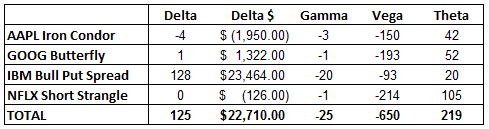
You can see that every position in this portfolio is short Vega, resulting in an overall Vega exposure of – 650.

This means that a roughly 1% increase in Implied Volatility will result in a $650 loss for this portfolio.

That might be above your risk tolerance, so you could look at swapping out one of the strategies.

Keep in mind that the volatility of each stock will perform differently.

For example, AAPL volatility may rise, while NFLX falls.

Your portfolio may not perform exactly as you would expect if you look at the total Vega number; you would need to also consider the individual stocks and their movements in Implied Volatility.

With that said, let’s look at the portfolio again, but this time, instead of the short strangle on NFLX, the trader is using a calendar spread.

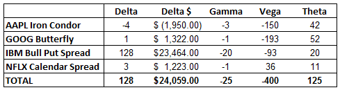
Here you can see the overall Vega exposure of the portfolio has dropped to -400, which is a significant reduction.

The overall Delta and Gamma have not changed.

The main trade-off in this case is the reduced Theta.

As you might have gathered, everything in options trading is a trade-off.

Generally, if you reduce your exposure to one variable, you will increase your exposure to another.

When trading options, it’s important to know the overall exposure of your positions, not just each individual position.

If you notice your portfolio is getting too long Vega, add some short Vega trades, and vice versa.

It can also be helpful to have pre-defined risk limits for Vega exposure, such as not letting your total Vega exposure get above ± 1000.

Implied Volatility And Option Strategies

Now that you have a good basic understanding of option volatility, you will appreciate that an individual option strategy has a particular exposure to volatility.

Certain strategies will benefit from a rise in Implied Volatility (positive position Vega) and others will benefit from a fall in volatility (negative Vega).

Most traders will typically prefer either to trade long Vega strategies, or short Vega.

As you can see in the graph below, volatility tends to gradually drift sideways / lower, and then shoot up over a short period of time.

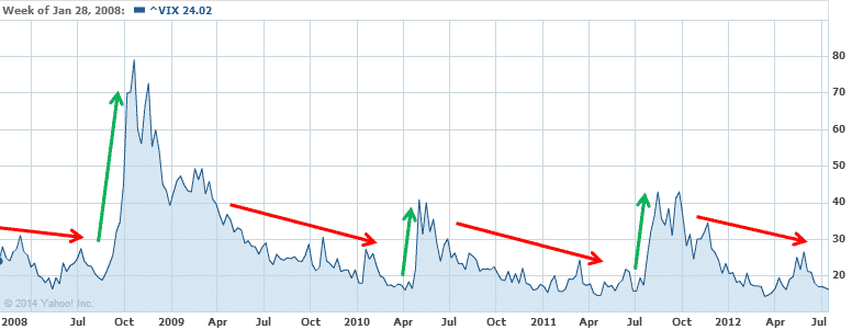
This situation occurs when there is a shock to the market.

Such things as a bad economic report, like GDP coming in well below expected, or a currency crisis, can result in a short, sharp spike in volatility, as traders panic and begin to close out positions.

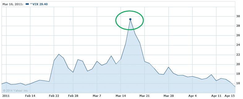
On March 11th, 2011, the tsunami in Japan caused the meltdown of the nuclear plant in Fukushima.

Take a look at the chart below and notice what happened to volatility over that period.

VIX traded steadily between 16 and 22 for the period shown, other than the brief spike up to 30 after the earthquake.

Mini market shocks like this occur pretty consistently each year.

This type of situation impacts long and short Vega traders very differently.

Every trader has their preference.

Some prefer to wait for these types of shock to occur in order to initiate short Vega trades; others like to have long Vega trades and wait for these events to occur.

Long Vega trades have a tendency to decay over time as volatility drifts sideways, so there is a cost of carry while these traders wait around for a market shock.

The advantage of long Vega trades is the huge potential to profit in a short period of time once volatility does spike.

Short Vega traders, on the other hand, can suffer rapid and painful losses on open trades when this situation occurs.

However, patient traders who wait for these events before initiating short Vega trades can do very well.

By March 21st, volatility had returned to somewhat normal levels and short Vega trades would have performed very well.

Your job is to figure out what side of the market you prefer to trade.

Some traders can trade both very well, but I think most traders find one side of the market easier to manage, based on their risk tolerance and personality.

My preference is short Vega trades; I find them much easier to manage than positions that slowly lose money each day due to time decay.

I’d much rather deal with the market shock when it occurs by closing or adjusting my short Vega trades.

While I do trade long Vega, I find it distinctly easier to trade short Vega.

How about you?

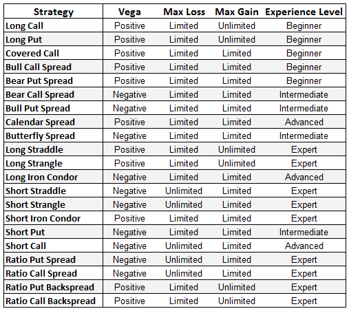
With that in mind, let’s look at some of the major option strategies and their Vega exposure:

FAQ

What Is Implied Volatility?

Implied volatility is a measure of the market’s expectation for the future volatility of a financial instrument, such as a stock or option.

It is derived from the market price of options on the instrument and reflects the perceived level of risk or uncertainty associated with the instrument’s future movements.

How Is Implied Volatility Calculated?

“Implied volatility is calculated using an options pricing model, such as the Black-Scholes model.

The model uses the market price of options and other inputs, such as the underlying price, strike price, time to expiration, and interest rates, to derive a theoretical value for the option.

By solving for the implied volatility input that makes the theoretical value match the market price, the implied volatility can be determined.

Why Is Implied Volatility Important?

Implied volatility is important because it can impact the price of options and other derivatives.

Higher implied volatility generally results in higher option prices, while lower implied volatility generally results in lower option prices.

Traders and investors can use implied volatility to help gauge the perceived risk or uncertainty in the market and make more informed trading decisions.

Conclusion

• Implied volatility is arguably THE most important concept for option traders to learn
• Just like a stock, traders should look to buy low implied volatility and sell high implied volatility
• You can gain an edge if your analysis of implied volatility is better than the consensus

Trade safe!

Disclaimer: The information above is for educational purposes only and should not be treated as investment advice. The strategy presented would not be suitable for investors who are not familiar with exchange traded options. Any readers interested in this strategy should do their own research and seek advice from a licensed financial adviser.